Frequency and Phase Modulation Systems

Module-driven study guide with original slide context preserved for full fidelity.

Module 1

Angle modulation foundations

Start with the carrier-angle viewpoint, the FM versus PM distinction, and the deviation relationships that everything else depends on.

Core frame

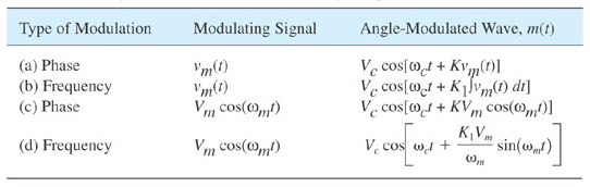
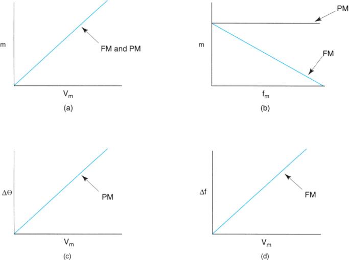
Angle modulation keeps carrier amplitude fixed

The deck opens by defining angle modulation as message-driven change in carrier phase. That single idea explains why FM and PM can suppress many amplitude-noise problems yet still force wider occupied bandwidth and more complex receiver design.

What the first chapter really tests

Separate classification from side effects

FM is classified by direct frequency control. PM is classified by direct phase control. Both create coupled phase and frequency behavior, but the direct control variable is what exam questions care about.

Formula discipline

Deviation and index are the first quantitative anchors

Slides 11 to 18 define deviation sensitivity, peak frequency deviation, percent modulation, and the modulation index relationships that reappear later when spectra and bandwidth are estimated.

Carrier model

s(t) = Vc cos(ωc t + θ(t))

Frequency deviation

Δf = Kf Vm

Modulation index

mf = Δf / fm

Source Material: Slides 1-18

Slide 1

Modulation and Encoding CE2280

Slide 2

Angle Modulation

Slide 3

FIGURE 7-1 Angle-modulated wave in the frequency domain.

Slide 4

Advantages of Angle Modulation

Slide 5

Disadvantages of Angle Modulation

Slide 6

Direct Phase Modulation

Slide 7

Direct Frequency Modulation

Slide 8

Difference Between FM and PM

Slide 9

FIGURE 7-2 Angle modulation in the time domain: (a) phase changing with time; (b) frequency changing with time

Slide 10

FIGURE 7-3 Phase and frequency modulation of a sine-wave carrier by a sine-wave signal: (a) unmodulated carrier; (b) modulating signal; (c) frequency-modulated wave; (d) phase-modulated wave

Slide 11

Deviation Sensitivity K1 (FM) K (PM)

Slide 12

TABLE 7-1 Equations for Phase- and Frequency-Modulated Carriers

Slide 13

Frequency Deviation

Slide 14

Percent Modulation

Slide 15

FIGURE 7-4 Relationship between modulation index, frequency deviation, and phase deviation in respect to modulations signal amplitude and frequency: (a) modulation index versus amplitude; (b) frequency deviation versus modulating frequency; (c) phase deviation versus amplitude; (d) frequency deviation versus amplitude

Slide 16

Tone Modulation

Slide 17

TABLE 7-2 Angle Modulation Summary

Slide 18

Example

Knowledge Check

Question 1

In direct FM, which output quantity is directly controlled by message amplitude?

Question 2

Calculate the percent modulation of an FM broadcast transmitter if the frequency deviation is 54 kHz. (Max deviation is 75 kHz). Enter the value as a percentage.

Module 2

Bessel functions and FM spectrum building

The second block explains why tone-modulated FM is not a one-sideband process. It is a carrier plus infinitely many sideband pairs weighted by Bessel coefficients.

Spectrum logic

The carrier and every sideband pair come from the same series

Slides 19 to 28 move from frequency analysis into Bessel coefficients, then into reading practical spectra. The exam skill is not memorizing every term but knowing how coefficient magnitude decides which lines matter.

Practical reading

Use the index first, then the table

Compute the modulation index, read the Bessel chart or table, keep significant coefficients, and place the resulting terms at fc ± nfm.

Series form

s(t) = Vc cos(ωc t + mf sin ωm t)

Placement rule

Sidebands occur at fc ± nfm

Table cue

Jn(mf) controls the nth sideband pair

Source Material: Slides 19-28

Slide 19

Frequency Analysis of Frequency Modulation

Slide 20

Bessel Function

Slide 21

Properties of the Bessel Function 1/2

Slide 22

Properties of the Bessel Function 2/2

Slide 23

TABLE 7-3 Bessel Functions of the First Kind, Jn(m)

Slide 24

FIGURE 7-5 Jn(m) versus m

Slide 25

Determining the Frequency Deviation

Slide 26

Example

Slide 27

FIGURE 7-6 Frequency spectrum

Slide 28

Frequency Spectrum

Knowledge Check

Question 1

What does a Bessel coefficient Jn(mf) tell you in tone-modulated FM?

Module 3

Bandwidth, deviation ratio, and FM power distribution

This chapter turns the spectrum picture into engineering decisions: classify low, medium, and high index FM, estimate occupied bandwidth, and understand why total FM power stays constant while redistribution changes.

Bandwidth estimation

Carson and 20 dB methods are both in play

Slides 29 to 40 treat bandwidth as something you estimate from deviation and modulating frequency, then confirm through spectrum or analyzer logic. The point is practical occupied spectrum, not an exact infinite-series count.

Power interpretation

FM power moves between carrier and sidebands without changing total transmit power

Slides 41 and 42 are easy to skip, but they are conceptually important. In ideal FM, amplitude is constant, so the total power is constant; what changes is where that power sits in the spectrum.

Carson rule

BW ≈ 2(Δf + fm)

Deviation ratio

DR = Δfmax / fm(max)

Classification cue

Low index < 1, medium 1 to 10, high index > 10

Source Material: Slides 29-42

Slide 29

Bandwidth Requirements of FM Waves

Slide 30

Classifications of FM Waveforms Low Index

Slide 31

Classifications of FM Waveforms Medium Index

Slide 32

Classifications of FM Waveforms High Index

Slide 33

Carson’s Rule

Slide 34

20 dB Method

Slide 35

Example

Slide 36

FIGURE 7-7 Frequency spectrum for Example 7-3

Slide 37

Deviation Ratio

Slide 38

Example

Slide 39

Example

Slide 40

FIGURE 7-8A Output frequency spectrums for Example 7-5: (a) frequency spectrums for FM and PM; (b) frequency spectrums for FM and PM; (c) frequency spectrum for FM; (d) frequency spectrum for PM

Slide 41

Average Power of a FM Wave 1/2

Slide 42

Average Power of a FM Wave 2/2

Knowledge Check

Question 1

Calculate the bandwidth (in kHz) using Carson's rule for a peak deviation of 50kHz and max modulating frequency of 10kHz.

Module 4

Broadcast FM services and preemphasis strategy

The next set of slides grounds FM in real service allocations and then focuses on preemphasis and deemphasis as a practical SNR-management technique.

Service context

FM is not one service with one bandwidth target

Slides 43 to 46 compare broadcast FM, TV audio, mobile, emergency, and amateur usage. The useful takeaway is that deviation and channel planning follow the service goal, not a single universal setting.

Noise shaping

Preemphasis lifts highs before transmission so deemphasis can recover them with better SNR

Slides 47 to 53 explain the standard reason preemphasis exists: high-frequency noise hurts more, so the transmitter boosts those components before modulation and the receiver restores the original balance afterward.

Transmit action

Boost high audio frequencies before FM modulation

Receive action

Apply reciprocal deemphasis after demodulation

Source Material: Slides 43-53

Slide 43

Commercial Broadcast Band FM Broadcast FM

Slide 44

Commercial Broadcast Band FM FM used in TV

Slide 45

Commercial Broadcast Band FM FM Used in Mobile or Emergency Services

Slide 46

Commercial Broadcast Band FM FM Used in Amateur Bands

Slide 47

Preemphasis and Deemphasis

Slide 48

FIGURE 7-13 FM signal-to-noise: (a) without preemphasis; (b) with preemphasis

Slide 49

Preemphasis Network

Slide 50

Deemphasis Network

Slide 51

FIGURE 7-14 Preemphasis and deemphasis: (a) schematic diagrams; (b) attenuation curves

Slide 52

FIGURE 7-15 Figure for Example 7-8: (a) S/N without preemphasis and deemphasis; (Continued)

Slide 53

FIGURE 7-15 (Continued) (b) S/N with preemphasis and deemphasis

Module 5

FM modulators, up-conversion, and transmitter building blocks

Slides 54 to 74 are an actual transmitter-design chapter, not a side note. They compare direct and indirect modulators, varactor and reactance methods, VCO approaches, and frequency translation techniques.

Hardware view

The deck walks through multiple ways to create FM

Simple direct FM, varactor-diode modulation, reactance modulators, and integrated VCO-based modulators are all here because each solves stability, deviation, or implementation cost differently.

Transmitter chain

Frequency multiplication and heterodyning reshape both carrier and deviation

The up-conversion and multiplication slides matter because they show how a low-frequency modulator can still become a stable high-frequency transmitter while preserving modulation behavior.

Stability control

PLL transmitters bridge crystal stability and wideband deviation

The PLL direct FM transmitter at the end of this block is one of the most practical slides in the whole analog section.

Design cue

Use frequency multiplication to scale both fc and Δf

Stability cue

PLL control keeps the VCO locked to a reference while preserving FM behavior

Source Material: Slides 54-74

Slide 54

Types of Frequency Modulators Direct FM

Slide 55

Types of Frequency Modulators InDirect FM

Slide 56

Frequency Modulators Simple Direct Modulator

Slide 57

FIGURE 7-16 Simple direct FM modulator

Slide 58

Frequency Modulators Varactor Diode Modulator 1/2

Slide 59

Frequency Modulators Varactor Diode Modulator 2/2

Slide 60

Varactor Diode

Slide 61

Varactor Diode Operation

Slide 62

Varactor Diode Applications

Slide 63

FIGURE 7-17 Varactor diode direct FM modulator

Slide 64

FIGURE 7-18 Varactor diode VCO FM modulator

Slide 65

Frequency Modulators Reactance Modulator

Slide 66

FIGURE 7-19 JFET reactance modulator: (a) schematic diagram; (b) ac equivalent circuit

Slide 67

Frequency Modulators LIC Direct Modulator

Slide 68

FIGURE 7-20 LIC direct FM modulator--simplified block diagram

Slide 69

Frequency Up-Conversion

Slide 70

Heterodyning Process

Slide 71

Frequency Multiplication

Slide 72

AFC LOOP

Slide 73

Frequency Transmitter PLL Direct FM Transmitter

Slide 74

FIGURE 7-26 Phase-locked-loop FM transmitter

Knowledge Check

Question 1

What does the acronym VCO stand for?

Module 6

FM receivers, detectors, and loop behavior

This module covers the receiver half of the analog chain: double-conversion FM receivers, detector choices, slope detection limits, PLL demodulation, and loop filter behavior.

Receiver chain

FM receivers are familiar until the detector stage

Slides 77 to 82 show that much of the RF and IF path resembles AM or superheterodyne practice, but the discriminator stage is what changes the system behavior.

Detector comparison

Slope detectors are simple, PLL detectors are robust

The deck contrasts slope detection with PLL demodulation. The exam-level takeaway is that slope detection is easy to explain but poor in linearity, while PLL demodulation tracks input deviation through a control loop.

Loop role

Phase comparator + LPF + VCO = tracking demodulator

LPF role

The loop filter sets acquisition and hold behavior

Source Material: Slides 77-90

Slide 77

FM Receivers 1/2

Slide 78

FM Receivers 2/2

Slide 79

FIGURE 8-1 Double-conversion FM receiver block diagram

Slide 80

Differences Between FM and AM Receivers

Slide 81

FM Demodulators 1/2

Slide 82

FM Demodulators 2/2

Slide 83

Slope Detector

Slide 84

FIGURE 8-2 Slope detector: (a) schematic diagram; (b) voltage-versus-frequency curve

Slide 85

Slope Detector Operation

Slide 86

Disadvantages of Slope Detector

Slide 87

PLL FM Demodulator

Slide 88

Operation of PLL

Slide 89

FIGURE 8-7 (a) Block diagram for a PLL FM demodulator; (b) PLL FM demodulator using the XR-2212 PLL

Slide 90

Properties of the LPF

Knowledge Check

Question 1

For an FM receiver with an input noise level of -112 dBm, postdetection SNR = 38 dB, FM improvement factor of 17 dB, and NF = 5 dB. Determine the minimum receive signal level in dBm.

Question 2

What type of demodulator is shown in this block diagram with a phase comparator, LPF, and VCO?

Module 7

Noise suppression, capture effect, stereo FM, and analog SNR

The remaining analog slides cover limiter behavior, thresholding, capture effect, stereo multiplexing, stereo recovery, and the analog SNR summary that closes the FM portion of the course.

Noise handling

Limiters and thresholding explain why FM gets quiet only above a useful input level

Slides 91 to 102 cover amplitude limiting, threshold behavior, and capture effect. This is the practical noise-performance chapter rather than a pure formula chapter.

Stereo multiplexing

Stereo FM is a composite baseband design problem

Slides 103 to 116 turn stereo broadcasting into a multiplexing problem: L + R baseband, L - R around 38 kHz, and a 19 kHz pilot so the receiver can rebuild the suppressed subcarrier.

Bridge to later chapters

The analog SNR slide closes the FM unit before the course shifts to digital communications

Slide 117 is a useful transition: signal-to-noise thinking remains important even when the course later moves into line coding, BER, and PCM.

Stereo baseband

Composite = (L + R) + pilot + DSB(L - R)

Capture cue

The stronger same-channel FM signal tends to dominate receiver output

Source Material: Slides 91-118

Slide 91

FM Noise Suppression

Slide 92

Amplitude Limiters

Slide 93

FIGURE 8-9 Amplitude limiter input and output waveforms: (a) input waveform; (b) output waveform

Slide 94

FIGURE 8-10 Limiter output: (a) captured by noise; (b) captured by signal

Slide 95

FM Thresholding

Slide 96

Limiter Circuits

Slide 97

FIGURE 8-12 Single-stage tuned limiter: (a) schematic diagram; (b) limiter action

Slide 98

FIGURE 8-13 Filtered limiter output

Slide 99

Cascaded Limiter Circuits

Slide 100

FM Capture Effect

Slide 101

Example

Slide 102

Example

Slide 103

FM Stereo Broadcasting

Slide 104

Composite Modulating Signal for Stereo FM

Slide 105

FIGURE 8-21 FM baseband spectrum: (a) prior to 1955; (b) prior to 1961; (c) since 1961

Slide 106

FM Stereo Transmission

Slide 107

FIGURE 8-22 Stereo FM transmitter using frequency-division multiplexing

Slide 108

Composite Stereo Waveform

Slide 109

TABLE 8-1 Composite FM Voltages

Slide 110

FIGURE 8-23 Development of the composite stereo signal for equal-amplitude L and R signals: (a) L audio signal; (b) R audio signal; (c) L + R stereo channel; (d) L - R stereo channel; (e) SCA + 19-kHz pilot; (f) composite baseband waveform

Slide 111

FIGURE 8-24 Development of the composite stereo signal for unequal-amplitude L and R signals: (a) L audio signal; (b) R audio signal; (c) L + R stereo channel; (d) L - R stereo channel; (e) SCA + 19-kHz pilot; (f) composite baseband waveform

Slide 112

FM Stereo Reception 1/2

Slide 113

FM Stereo Reception 2/2

Slide 114

FIGURE 8-25 FM stereo and mono receiver

Slide 115

FIGURE 8-26 Stereo matrix network decoder

Slide 116

Deemphasis Network

Slide 117

S/N for analog systems

Slide 118

Summary

Knowledge Check

Question 1

In FM Stereo Broadcasting, what is the frequency of the pilot subcarrier in kHz?

Module 8

Digital communications foundations, coding, and line signaling

This block deserves a full module, not a review footnote. It introduces digital transmission versus digital radio, information capacity, character coding, error detection, ARQ, channel coding, and line-code synchronization issues.

Big distinction

Digital transmission and digital radio are not the same thing

Slides 120 to 138 separate direct pulse transmission on guided media from digital information sent on a modulated analog carrier through space. That distinction sets up the later digital-radio modules.

Capacity and coding

Information theory sets the ceiling before implementation choices start

Slides 139 to 147 move through information capacity, Shannon thinking, and BER reference figures. Then the deck shifts into symbol definitions, baud rate, Nyquist-rate ideas, and character coding such as ASCII and EBCDIC.

Reliability layer

Error detection, ARQ, channel coding, and line codes are all part of the source context

Slides 169 to 197 cover parity, CRC, retransmission logic, block and convolutional coding, and the synchronization constraints behind AMI-family line codes.

Capacity cue

Shannon capacity grows with bandwidth and SNR

Nyquist cue

Binary data rate in an ideal noiseless channel relates to available bandwidth

Synchronization cue

Long-distance digital links need self-clocking or recovered timing

Source Material: Slides 119-197

Slide 119

Modulation and Encoding CE2280

Slide 120

Transfer of information from one point to another using digital methods

Slide 121

Transmission of digital pulses (marks and spaces) between any number of stations in a communications system over one of the following transmission mediums:

Slide 122

PAM pulse amplitude modulation

Slide 123

Figure only.

Slide 124

Figure only.

Slide 125

Figure only.

Slide 126

Figure only.

Slide 127

Digital Transmission

Slide 128

Transmission of a digitally modulated analog carrier between two stations in a communications system using free space as the transmission media

Slide 129

ASK Amplitude Shift Keying

Slide 130

Figure only.

Slide 131

Figure only.

Slide 132

Figure only.

Slide 133

Quadrature Phase Shift Keying

Slide 134

QAM

Slide 135

Digital Radio

Slide 136

Mismatched system

Slide 137

Transmission quality is almost independent of the distance between terminals

Slide 138

Increased bandwidth requirement

Slide 139

Measure of how much information can be propagated through a communications system

Slide 140

In information theory, this tells the maximum rate at which information can be transmitted over a communications channel of a specified bandwidth in the presence of noise.

Slide 141

In information theory, the noisy-channel coding theorem, establishes that for any given degree of noise contamination of a communication channel, it is possible to communicate discrete data (digital information) nearly error-free up to a computable maximum rate through the channel.

Slide 142

Hartley’s Law

Slide 143

For a standard telephone circuit with a signal-to-noise power ratio of 1023 (60 dB) and a bandwidth of 3 kHz, the Shannon limit for information capacity is :

Slide 144

P(e) vs. C/N

Slide 145

FIGURE 9-48 Error rates of PSK modulation systems

Slide 146

FIGURE 9-49 Error rates of QAM modulation systems

Slide 147

FIGURE 9-50 Error rates for FSK modulation systems

Slide 148

Represents a digit that corresponds to the number of conditions, levels, or combinations possible for a given number of binary variables

Slide 149

Figure only.

Slide 150

Figure only.

Slide 151

Rate of change of the digital information signal, which is binary

Slide 152

Unit of transmission rate, modulation rate or symbol rate

Slide 153

Figure only.

Slide 154

Also called the Nyquist frequency

Slide 155

character codes

Slide 156

American Standard Code for Information Interchange

Slide 157

Figure only.

Slide 158

Figure only.

Slide 159

TABLE 22-2 ASCII-77: Odd Parity

Slide 160

TABLE 22-2 (Continued)

Slide 161

Figure only.

Slide 162

8 bit version of ASCII resulting in more control characters, foreign letters and punctuations.

Slide 163

Extended ASCII Code Extra Characters

Slide 164

Figure only.

Slide 165

Extended Binary Coded Decimal Interchange Code

Slide 166

TABLE 22-3 EBCDIC Code

Slide 167

TABLE 22-3 (Continued)

Slide 168

TABLE 22-3 (Continued)

Slide 169

produced by external (EMI/RFI) or internal noise (thermal)

Slide 170

process of monitoring the received data and determining when a transmission error occurs

Slide 171

character must contain either an odd number of Marks (odd parity) or an even number of Marks (even parity)

Slide 172

FIGURE 22-7 Asynchronous data format

Slide 173

2. Horizontal Redundancy Checking (HRC)

Slide 174

3. HRC and VRC Simultaneously

Slide 175

Used with asynchronous or synchronous communications

Slide 176

Cyclic code

Slide 177

FIGURE 22-5 CRC-16 generating circuit

Slide 178

Determining what to do with the data that contains errors

Slide 179

automatic request for retransmission (ARQ)

Slide 180

Uses acknowledgments to indicate the successful or unsuccessful reception of data

Slide 181

Selective repeat

Slide 182

Channel Coding

Slide 183

Block codes

Slide 184

Convolutional codes

Slide 185

Frequently used in digital communication and storage systems to improve the performance of forward error correcting codes.

Slide 186

In multi-carrier communication systems, interleaving across carriers may be employed to provide frequency diversity, e.g., to mitigate frequency-selective fading or narrowband interference.

Slide 187

series of pulses consisting of Marks and Space

Slide 188

Space remains at zero volts and Mark remains at a positive voltage for the duration of a bit time

Slide 189

Space remains at negative voltage and Mark remains at a positive voltage for the duration of a bit time

Slide 190

Mark will be a positive voltage or a Space will be a zero volts for the first half of the bit time

Slide 191

Mark will be a positive voltage or a Space will be a negative voltage for the first half of the bit time

Slide 192

Mark is defined as a positive to negative transition at the center of each bit time

Slide 193

transition each time a Mark occurs by inverting the signal amplitude for the first half of the bit time. The second half will be zero volts

Slide 194

Figure only.

Slide 195

Other AMI Line Codes (B8ZS)

Slide 196

Other AMI Line Codes (B6ZS)

Slide 197

Other AMI Line Codes (B3ZS)

Knowledge Check

Question 1

What is the most common error detection method that uses binary division by a constant? (Abbreviation)

Question 2

What does ARQ stand for?

Question 3

What is the main distinction between digital transmission and digital radio in this deck?

Module 9

Digital radio introduction, FSK, and ASK

The digital-modulation chapter begins with radio-system context and then spends real time on FSK and ASK transmitters, detectors, and coherent versus noncoherent reception.

FSK first

FSK is the direct digital relative of FM thinking

Slides 203 to 223 show why FSK is a natural starting point after the analog FM chapter: marks and spaces become distinct carrier frequencies, and the deck compares continuous and discontinuous implementations plus coherent and noncoherent detection.

ASK contrast

ASK is simpler conceptually but more exposed to amplitude noise

Slides 224 to 233 position ASK as digital amplitude modulation and use that contrast to motivate why phase-based and quadrature methods often perform better.

FSK cue

Binary states map to different carrier frequencies

ASK cue

Binary states map to different carrier amplitudes

Detection cue

Coherent receivers need a carrier/timing reference; noncoherent receivers trade complexity for performance

Source Material: Slides 198-233

Slide 198

Modulation and Encoding CE2280

Slide 199

Systems where relatively high frequency analog carriers are modulated by relatively low frequency digital information systems.

Slide 200

FIGURE 9-1 Simplified block diagram of a digital radio system

Slide 201

FIGURE 22-27 Data communications modems - POTS analog channel

Slide 202

transmission of a digitally modulated analog carrier over the earth’s atmosphere

Slide 203

Frequency Shift Keying (FSK)

Slide 204

FM(t) = AC cos ( wCt + mf sin wmt )

Slide 205

FIGURE 9-4A FSK in the time domain: (a) waveform; (b) truth table

Slide 206

FIGURE 9-4B FSK in the time domain: (a) waveform; (b) truth table

Slide 207

FIGURE 9-3 FSK in the frequency domain

Slide 208

Abrupt FSK

Slide 209

FIGURE 9-10 Noncontinuous FSK waveform

Slide 210

FIGURE 9-11 Continuous-phase MSK waveform

Slide 211

consist of a VCO:

Slide 212

Figure only.

Slide 213

FIGURE 9-6 FSK modulator

Slide 214

TABLE 7-2 Angle Modulation Summary

Slide 215

Fundamental frequency of binary input

Slide 216

FIGURE 9-5 FSK modulator, tb, time of one bit = 1/fb; fm, mark frequency; fs, space frequency; T1, period of shortest cycle; 1/ T1, fundamental frequency of binary square wave; fb, input bit rate (bps)

Slide 217

Figure only.

Slide 218

consist of a PLL

Slide 219

FIGURE 9-9 PLL-FSK demodulator

Slide 220

FIGURE 9-8 Coherent FSK demodulator

Slide 221

consist of BPF, full-wave rectifier, LPF and pulse shaper

Slide 222

FIGURE 9-7 Noncoherent FSK demodulator

Slide 223

Figure only.

Slide 224

Amplitude Shift Keying (ASK)

Slide 225

AM(t) = AC ( 1 + μ xm(t) ) cos wct

Slide 226

Continuous carrier

Slide 227

FIGURE 9-2 Digital amplitude modulation: (a) input binary; (b) output DAM waveform

Slide 228

consist of a summer and a balanced modulator

Slide 229

FIGURE 9-13 (a) Balanced ring modulator; (b) logic 1 input; (c) logic 0 input

Slide 230

carrier / CLK frequency used in the receiver is of the same phase and frequency as the carrier used in the transmitter

Slide 231

Figure only.

Slide 232

noncoherent

Slide 233

Figure only.

Knowledge Check

Question 1

What digital modulation technique is represented by this waveform where the carrier amplitude shifts between a high and low level?

Module 10

PSK, QPSK, QAM, carrier recovery, and BER tradeoffs

This is another major chapter. It covers BPSK, QPSK, QAM, coherent recovery loops, clock recovery, trellis coding, and BER comparisons across schemes.

Phase family

PSK uses phase states because they hold up better in noise-limited links

Slides 234 to 252 move from BPSK into QPSK transmitters and receivers. The essential study point is that multilevel phase states improve bit efficiency at the cost of tighter recovery requirements.

Quadrature scaling

QAM combines phase and amplitude to raise information density

Slides 253 to 263 use 8-QAM as the teaching example, then compare efficiency across ASK, FSK, PSK, and QAM families.

Recovery and performance

Carrier recovery, clock recovery, trellis coding, and BER are part of the same design conversation

Slides 264 to 292 show why high-order digital modulation is not just about constellations. The receiver must rebuild timing and carrier references accurately enough to achieve the expected BER.

QPSK cue

Two input bits select one of four phase states

QAM cue

I/Q components change both amplitude and phase

Performance cue

Higher spectral efficiency usually demands higher SNR and tighter recovery

Source Material: Slides 234-292

Slide 234

Phase Shift Keying (PSK)

Slide 235

PM(t) = AC cos ( wCt + mp cos wmt )

Slide 236

consist of balance modulator which acts as a phase reversal switch and BPF

Slide 237

FIGURE 9-12 BPSK transmitter

Slide 238

FIGURE 9-15 Output phase-versus-time relationship for a BPSK modulator

Slide 239

FIGURE 9-14 BPSK modulator: (a) truth table; (b) phasor diagram; (c) constellation diagram

Slide 240

Synchronous PSK Demodulator

Slide 241

FIGURE 9-16 Block diagram of a BPSK receiver

Slide 242

Figure only.

Slide 243

Quadrature Phase Shift Keying

Slide 244

consist of a bit splitter, an I (in-phase) channel and a Q (quadrature) channel sections, linear summer, and BPF

Slide 245

FIGURE 9-17 QPSK modulator

Slide 246

IQ Modulator Basics(335)

Slide 247

I active above with no Q (BPSK)

Slide 248

FIGURE 9-18 QPSK modulator: (a) truth table; (b) phasor diagram; (c) constellation diagram

Slide 249

FIGURE 9-19 Output phase-versus-time relationship for a QPSK modulator

Slide 250

FIGURE 9-20 Bandwidth considerations of a QPSK modulator

Slide 251

Synchronous

Slide 252

FIGURE 9-21 QPSK receiver

Slide 253

Quadrature Amplitude Modulation

Slide 254

Eight Quadrature Amplitude Modulation

Slide 255

consist of a bit splitter, DAC, I channel and Q channel section, linear summer and BPF

Slide 256

FIGURE 9-30 8-QAM transmitter: (a) block diagram; (b) truth table 2-4 level converters

Slide 257

FIGURE 9-31 8-QAM modulator: (a) truth table; (b) phasor diagram; (c) constellation diagram

Slide 258

FIGURE 9-32 Output phase and amplitude-versus-time relationship for 8-QAM

Slide 259

consist of power splitter, PLL, I channel and Q channel section, ADC and shift register

Slide 260

8QAM Demodulator

Slide 261

TABLE 9-1 ASK, FSK, PSK, and QAM Summary

Slide 262

Information density or spectral efficiency

Slide 263

TABLE 9-2 ASK, FSK, PSK, and QAM Summary

Slide 264

Phase referencing

Slide 265

Common method of achieving carrier recovery for BPSK

Slide 266

FIGURE 9-37 Squaring loop carrier recovery circuit for a BPSK receiver

Slide 267

Quadrature Loop

Slide 268

FIGURE 9-38 Costas loop carrier recovery circuit

Slide 269

Digital radio requires precise timing or clock synchronization between the transmitter and the receiver circuitry

Slide 270

FIGURE 9-40 (a) Clock recovery circuit; (b) timing diagram

Slide 271

Used in telephony circuit modems to reduce SNR required to transmit data

Slide 272

FIGURE 9-43 QPSK constellations: (a) standard encoding format; (b) trellis encoding format

Slide 273

FIGURE 9-44 8-PSK TCM constellations

Slide 274

TABLE 9-3 Trellis Coding Gain

Slide 275

FIGURE 9-45 128-Point QAM TCM constellation

Slide 276

FIGURE 9-46 One-fourth of a 960-Point QAM TCM constellation

Slide 277

No, C/N, and C/No

Slide 278

Errors

Slide 279

Theoretical ( mathematical) expectation of the bit error rate for a given system

Slide 280

A measure of transmission quality and the ability of a receiver to correctly extract the original information from among the noise in the received signal.

Slide 281

In a communication system, the receiver side BER may be affected by:

Slide 282

Transmission BER

Slide 283

BERT

Slide 284

Pattern generator, which transmits a defined test pattern to the DUT or test system

Slide 285

TABLE 9-4 Performance Comparison of Various Digital Modulation Schemes (BER = 10-6)

Slide 286

Figure only.

Slide 287

FIGURE 9-48 Error rates of PSK modulation systems

Slide 288

QAM BER Results

Slide 289

FIGURE 9-49 Error rates of QAM modulation systems

Slide 290

FIGURE 9-50 Error rates for FSK modulation systems

Slide 291

QPSK BER Results

Slide 292

P(e) vs. C/N

Knowledge Check

Question 1

What type of digital modulation constellation is shown here?

Question 2

What is the process of extracting a phase coherent reference carrier from a receiver signal called?

Module 11

Digitizing analog signals: sampling, aliasing, PAM, PWM, and PPM

The course then pivots from digital carriers to digitizing analog sources. This block covers why digital pulses are robust, how sampling works, and how pulse-modulation families differ before full PCM coding begins.

System reason

Digitizing analog signals is a transport pipeline, not one isolated formula

Slides 293 to 299 frame digitization as three steps: sample the analog signal, turn samples into discrete pulses, and transport those pulses through a physical medium.

Sampling theorem

Nyquist and aliasing are central, not optional review points

Slides 301 to 322 walk through natural sampling, flat-top sampling, aperture error, Nyquist sampling, and aliasing in both time and frequency domains.

Pulse families

PWM, PPM, PAM, and PCM are related but not interchangeable

Slides 323 to 331 map the pulse-modulation family so the later PCM chapter has context.

Sampling theorem

fS ≥ 2fa

Aliasing cue

If fS < 2fa, the original message cannot be reconstructed cleanly

Source Material: Slides 293-331

Slide 293

Modulation and Encoding CE2280

Slide 294

Transmittal of digital signals between two or more points in a communications system

Slide 295

Noise immunity

Slide 296

More resistant to additive noise

Slide 297

Requires more bandwidth

Slide 298

Sampling analog information signals

Slide 299

Process in which a message is sampled at regular intervals and each sample is proportional to the amplitude of the message at the time of the sample

Slide 300

Figure only.

Slide 301

Amplitude of each sample pulse follows the message signal during the pulse width time of the sampling signal

Slide 302

FIGURE 10-3 Natural sampling: (a) input analog signal; (b) sample pulse; (c) sampled output

Slide 303

Figure only.

Slide 304

Rectangular pulses whose amplitudes represent the message signal at particular point in the sample interval (beginning or middle or end)

Slide 305

FIGURE 10-4 Flat-top sampling: (a) input analog signal; (b) sample pulse: (c) sampled output

Slide 306

Figure only.

Slide 307

Purpose is to periodically sample the continually changing analog input voltage and convert those samples to a series of constant amplitude PAM voltage levels

Slide 308

PAM Power Supplies: Dual Polarity

Slide 309

PAM Power Supplies: Single Polarity

Slide 310

Any bandlimited signal does not need to be continuously transmitted in order to retain all its information content. No information is lost in such a signal if it is sampled at regular intervals of time at a rate equal to or higher than twice the highest frequency component of the message. The signal can be reconstructed by passing it through a LPF.

Slide 311

fS ≥ 2 fa

Slide 312

Time Domain Representation: fS < 2 fa

Slide 313

Time Domain Representation: fS = fa

Slide 314

Time Domain Representation: fS = 2 fa

Slide 315

Time Domain Representation: fS > 2 fa

Slide 316

Frequency Domain Representation: fS > 2 fa

Slide 317

Frequency Domain Representation: fS = 2 fa

Slide 318

Frequency Domain Representation: fS < 2 fa

Slide 319

FIGURE 10-6 Output spectrum for a sample-and-hold circuit: (a) no aliasing; (b) aliasing distortion

Slide 320

Example 15-2

Slide 321

FIGURE 10-7 Output spectrum for Example 15-2

Slide 322

fS > 2 fa

Slide 323

Pulse Duration Modulation

Slide 324

Figure only.

Slide 325

Figure only.

Slide 326

Process in which fixed width, fixed amplitude pulses vary their position proportional to the change in the message amplitude

Slide 327

PPM is produced from PWM

Slide 328

Figure only.

Slide 329

Lab Circuit

Slide 330

Figure only.

Slide 331

FIGURE 10-1 Pulse modulation: (a) analog signal; (b) sample pulse; (c) PWM; (d) PPM; (e) PAM; (f) PCM

Knowledge Check

Question 1

This output spectrum shows the effects of sampling. What phenomenon causes the overlapping of spectral components if fs < 2fa?

Question 2

A signal has a maximum frequency of 4kHz. According to the Nyquist sampling theorem, what is the minimum sampling rate in kHz?

Module 12

PCM, quantization, dynamic range, and companding

Slides 332 to 381 form a full PCM chapter: encoder blocks, quantization, quantization noise, resolution, dynamic range, coding efficiency, data rate, linear versus nonlinear coding, and analog and digital companding.

PCM chain

The encoder-decoder path matters as much as the formulas

The simplified PCM system and its BPF, line driver, serial/parallel logic, and code structure give the hardware view that the quantization formulas depend on.

Quantization study core

Resolution, error, dynamic range, and SQNR are the main numeric ideas

Slides 339 to 359 are the core quantitative study block. They explain why more bits reduce quantum size, improve signal representation, and raise recoverable dynamic range.

Companding

Companding exists because low-amplitude signal accuracy matters

Slides 360 to 381 explain analog and digital companding, μ-law, A-law, and the tradeoff between compression efficiency and introduced error.

Resolution cue

Smaller quantum size means finer amplitude representation

Data-rate cue

PCM line rate depends on sample rate and bits per sample

Companding cue

Nonlinear coding improves small-signal representation at the cost of nonuniform error

Source Material: Slides 332-381

Slide 332

Preferred method of communications within the public switched telephony network

Slide 333

FIGURE 10-2 Simplified block diagram of a single-channel, simplex PCM transmission system

Slide 334

BPF

Slide 335

S/P

Slide 336

Line Driver

Slide 337

N-bit binary code

Slide 338

TABLE 10-1 Three-Bit PCM Code

Slide 339

Process of converting an infinite number of possibilities to a finite number of conditions

Slide 340

Quantization range for each code is equal to plus or minus one half the magnitude of a quantum except for positive zero and negative zero

Slide 341

TABLE 10-2 Three-Bit PCM Code

Slide 342

Quantization Noise

Slide 343

FIGURE 10-8 (a) Analog input signal; (b) sample pulse; (c) PAM signal; (d) PCM code

Slide 344

FIGURE 10-9 PAM: (a) input signal; (b) sample pulse; (c) PAM signal

Slide 345

Reduce the magnitude of the quantum

Slide 346

FIGURE 10-10 Linear input-versus-output transfer curve: (a) linear transfer function; (b) quantization; (c) Qe

Slide 347

Resolution

Slide 348

Quantization Error

Slide 349

Dynamic Range

Slide 350

Two codes representing zero

Slide 351

TABLE 10-3 Dynamic Range versus Number of PCM Magnitude Bits

Slide 352

Coding Efficiency

Slide 353

Signal to quantization noise ratio

Slide 354

For linear system

Slide 355

Divide voltage of the sample by the resolution

Slide 356

Data rate at which serial PCM bits are clocked out of the PCM encoder onto the transmission line

Slide 357

Example 1/2

Slide 358

Find the following:

Slide 359

For a linear PCM with the following parameters:

Slide 360

Linear Coding

Slide 361

Nonlinear Coding

Slide 362

FIGURE 10-11 (a) Linear versus (b) nonlinear encoding

Slide 363

Used to produce non-linear PCM codes

Slide 364

FIGURE 10-13 Basic companding process

Slide 365

In the encoder

Slide 366

FIGURE 10-14 PCM system with analog companding

Slide 367

Used for voice communications in the United States and Japan

Slide 368

FIGURE 10-15 -law compression characteristics

Slide 369

Figure only.

Slide 370

Used for voice communications in Europe

Slide 371

Figure only.

Slide 372

In the encoder

Slide 373

FIGURE 10-16 Digitally companded PCM system

Slide 374

12 bit to 8 bit digital compression

Slide 375

FIGURE 10-17 255 compression characteristics (positive values only)

Slide 376

Figure only.

Slide 377

FIGURE 10-18 12-bit-to-8-bit digital companding: (a) 8-bit 255 compressed code format; (b) 255 encoding table; (c) 255 decoding table

Slide 378

Figure only.

Slide 379

ADC produces a 12 bit sign-magnitude code

Slide 380

MSB bit of the 8 bit code is reinserted at the decoder as the sign bit for the 12 bit code

Slide 381

Magnitude of the compression error is not the same for all samples

Module 13

TDM, PCM/TDM systems, and carrier hierarchies

This chapter is the multiplexing and telephony-systems block: TDM slotting, frame timing, PCM/TDM transport, T1 framing, fractional T1, and North American and European hierarchy summaries.

Multiplexing idea

TDM shares one path by interleaving channels in time

Slides 382 to 393 are the system-level explanation for why multiple analog or digital channels can share one facility without simultaneous overlap.

Carrier systems

T1 and E-carrier details are part of the actual final-review content

Slides 401 to 417 go beyond abstract TDM and into concrete hierarchy, framing, signaling-channel, and line-interface details used in telephony systems.

Frame cue

Frame time is set by the channel sampling schedule

DS-0 cue

A standard voice PCM channel becomes the building block of larger hierarchies

Source Material: Slides 382-417

Slide 382

Immune to noise

Slide 383

Transmission from multiple sources occur on the same facility but not at the same time

Slide 384

Figure only.

Slide 385

Time interval; during which the common transmission path is allocated to a particular communication channel

Slide 386

Time it takes to transmit one sample from each communications channel

Slide 387

Transmission from various sources are interleaved in the time domain

Slide 388

PAM\TDM Encoder

Slide 389

Figure only.

Slide 390

PAM\TDM Decoder

Slide 391

Figure only.

Slide 392

Two or more message channels are sampled, converted to PCM codes, and then time division multiplexed onto a single metallic or optical fiber cable

Slide 394

Two transduces are to be PCM/TDM together and transmitted to a industrial control room. The following is the specifications for the PCM/TDM system:

Slide 395

Used in voice communications

Slide 396

FIGURE 11-1 Single-channel (DS-0-level) PCM transmission system

Slide 397

FIGURE 11-1 Single-channel (DS-0-level) PCM transmission system

Slide 398

FIGURE 11-2A Two-channel PCM-TDM system: (a) block diagram;

Slide 399

FIGURE 11-2B Two-channel PCM-TDM system: (b) TDM frame

Slide 400

FIGURE 11-2 Two-channel PCM-TDM system: (a) block diagram;

Slide 401

Communications system that uses digital pulses rather than analog signals to encode information

Slide 402

T1 stands for transmission one

Slide 403

FIGURE 11-3A Bell system T1 digital carrier system: (a) block diagram;

Slide 404

FIGURE 11-3B Bell system T1 digital carrier system: (b) sampling sequence

Slide 405

Line driver provides:

Slide 406

FIGURE 11-3A Bell system T1 digital carrier system: (a) block diagram

Slide 407

Line Receiver provides:

Slide 408

FIGURE 11-7A Framing bit circuitry T1 carrier system: (a) DS-1

Slide 409

FIGURE 11-7B Framing bit circuitry T1 carrier system: (b) DS-1C

Slide 410

Distributes the channels in a standard T1 system among more than one user, allowing several subscribers to share one T1 line: both its capacity and its cost

Slide 411

FIGURE 11-8 Fractional T1 carrier service

Slide 412

Used for multiplexing digital signals from multiple sources into a single higher speed pulse stream suitable for transmission on the next higher level of the hierarchy

Slide 413

FIGURE 11-9 North American Digital Hierarchy

Slide 414

TABLE 11-2 North American Digital Hierarchy Summary

Slide 415

E- lines

Slide 416

FIGURE 11-19 CCITT TDM frame alignment and common signaling channel alignment: (a) CCITT TDM frame (125 s, 256 bits, 2.048 Mbps); (b) common signaling channel

Slide 417

TABLE 11-5 European Transmission Rates and Capacities

Knowledge Check

Question 1

A T1 digital carrier system time division multiplexes 24 voice band channels. If each frame contains 193 bits and the frame rate is 8000 frames/second, what is the line speed in Mbps?

Module 14

Delta modulation, pulse impairments, and eye diagrams

The closing slides are not throwaway material. They cover delta modulation behavior, its encoder and decoder, slope overload, granular noise, and the pulse-shape impairments diagnosed with eye diagrams.

Delta logic

Delta modulation sends change direction instead of full PCM words

Slides 418 to 432 explain why delta modulation can use lower bit rates and lower power than full PCM while introducing its own failure modes.

Failure modes

Slope overload and granular noise are the two named distortions to remember

These slides explicitly contrast fast-changing inputs that outrun the staircase with slow-changing inputs that create granular jitter around the true value.

Transmission quality

Eye diagrams turn pulse distortion into a visual diagnostic

Slides 433 to 439 close the deck with timing inaccuracy, amplitude distortion, ISI, and eye-diagram interpretation, which is useful for understanding digital pulse quality after a real channel.

Slope overload cue

Occurs when the signal changes faster than the staircase can track

Granular-noise cue

Occurs when step changes are too coarse for slowly varying input

Eye-diagram cue

A more open eye indicates better timing margin and less ISI

Source Material: Slides 418-439

Slide 418

Single bit PCM code

Slide 419

FIGURE 10-21 Ideal operation of a delta modulation encoder

Slide 420

Idling

Slide 421

Slope overload

Slide 422

Input analog signal is sampled and converted to a staircase PAM signal

Slide 423

FIGURE 10-20 Delta modulation transmitter

Slide 424

Initially the up down counter is zeroed

Slide 425

Decoder is almost identical to the encoder except for the comparator

Slide 426

FIGURE 10-22 Delta modulation receiver

Slide 427

More prevalent in analog signals that have steep slopes or whose amplitudes vary rapidly

Slide 428

FIGURE 10-23 Slope overload distortion

Slide 429

More prevalent in analog signals that have gradual slopes and whose amplitudes vary only a small amount

Slide 430

FIGURE 10-24 Granular noise

Slide 431

Requires no synchronization

Slide 432

Delta can not be integrated with other digital signals: multiplexed

Slide 433

Interference from other impulses appear during the sampling instant

Slide 434

FIGURE 10-29 Pulse response: (a) NRZ input signal; (b) output from a perfect filter; (c) output from an imperfect filter

Slide 435

Timing inaccuracies

Slide 436

Amplitude distortion

Slide 437

Convenient technique for determining the effects of the degradations introduced into the pulses as they travel to the regenerator

Slide 438

FIGURE 10-30 Eye diagram measurement setup

Slide 439

FIGURE 10-31 Eye diagram

Knowledge Check

Question 1

What is the primary advantage of Delta Modulation over standard PCM?

Question 2

What problem is caused when a delta modulator staircase cannot follow a rapidly changing input?

Question 3

What is the name of this diagnostic display used to evaluate digital pulse quality?

Module 15

Mixed final test checkpoint

This checkpoint spans the analog and digital halves of the deck. Grade it only after you have worked through the source-backed modules above.

Question 1

In direct FM, which output quantity is directly controlled by message amplitude?

Question 2

What does the acronym VCO stand for?

Question 3

What type of digital modulation constellation is shown here?

Question 4

Calculate the bandwidth (in kHz) using Carson's rule for a peak deviation of 50kHz and max modulating frequency of 10kHz.

Question 5

What is the primary advantage of Delta Modulation over standard PCM?

Question 6

What is the most common error detection method that uses binary division by a constant? (Abbreviation)

Question 7

This output spectrum shows the effects of sampling. What phenomenon causes the overlapping of spectral components if fs < 2fa?

Question 8

A signal has a maximum frequency of 4kHz. According to the Nyquist sampling theorem, what is the minimum sampling rate in kHz?

Question 9

What problem is caused when a delta modulator staircase cannot follow a rapidly changing input?

Question 10

In FM Stereo Broadcasting, what is the frequency of the pilot subcarrier in kHz?

Question 11

What is the name of this diagnostic display used to evaluate digital pulse quality?

Question 12

For an FM receiver with an input noise level of -112 dBm, postdetection SNR = 38 dB, FM improvement factor of 17 dB, and NF = 5 dB. Determine the minimum receive signal level in dBm.

Question 13

What does a Bessel coefficient Jn(mf) tell you in tone-modulated FM?

Question 14

What does ARQ stand for?

Question 15

What type of demodulator is shown in this block diagram with a phase comparator, LPF, and VCO?

Question 16

A T1 digital carrier system time division multiplexes 24 voice band channels. If each frame contains 193 bits and the frame rate is 8000 frames/second, what is the line speed in Mbps?

Question 17

What is the main distinction between digital transmission and digital radio in this deck?

Question 18

What is the process of extracting a phase coherent reference carrier from a receiver signal called?

Question 19

What digital modulation technique is represented by this waveform where the carrier amplitude shifts between a high and low level?

Question 20

Calculate the percent modulation of an FM broadcast transmitter if the frequency deviation is 54 kHz. (Max deviation is 75 kHz). Enter the value as a percentage.